Seedling and Sapling Survival and Recruitment: Traits, Environment and Demography
2026-10-31
This report summarises the cleaned census, trait and environmental data, the species trait estimates and their uncertainty, the trait and environmental PCAs, and the fitted survival (mortality) and recruitment models. All numbers and figures are read from the outputs of the analysis scripts; nothing is refitted when the report is knitted.
Workflow. 1_clean.R (cleaning) →
2_standardise.R (species trait estimation and
standardisation) → 3_explore.R (descriptive figures, trait
coverage and reliability) → 4_dag.R (causal DAGs) →
5_pca.R (trait and environmental PCAs) →
models/model_1.R … model_6.R.
./run.sh runs the whole pipeline. A section that shows
“Output not found” means the corresponding script has not been run since
the outputs changed.
1 Data
1.1 Census
The cleaned census has 38,731 records from 8 census dates, covering 10,184 individuals of 90 species in 250 plots across 6 sites. Each record is an individual’s status at one census (recruited, survived or died); records run from an individual’s first appearance to its first recorded death.
| Date | recruited | died | survived | Total |
|---|---|---|---|---|
| 2021-11-01 | 3809 | 0 | 0 | 3809 |
| 2022-04-01 | 1053 | 1162 | 2646 | 4861 |
| 2022-11-01 | 2426 | 891 | 2807 | 6124 |
| 2023-05-01 | 368 | 1707 | 3526 | 5601 |
| 2023-11-01 | 1178 | 679 | 3204 | 5061 |
| 2024-03-01 | 409 | 1018 | 3365 | 4792 |
| 2024-11-01 | 839 | 799 | 2975 | 4613 |
| 2025-03-01 | 57 | 741 | 3072 | 3870 |
Record counts describe survey effort as much as demography: they change with deaths, recruitment and survey coverage, so they are not survival rates.
| Census | New individuals tagged |
|---|---|
| nov21 | 3836 |
| apr22 | 1053 |
| nov22 | 2426 |
| may23 | 368 |
| nov23 | 1180 |
| mar24 | 409 |
| nov24 | 841 |
| mar25 | 57 |
Each site’s first census tags every plant present, so those counts are baseline inventories rather than recruits; the recruitment summaries and models drop each site’s first census. Large changes between later censuses, particularly at the most recent census, could reflect real recruitment change or incomplete tagging, and the census data alone cannot tell these apart.
Age is counted from an individual’s recorded cohort. Individuals already present at a site’s first census are assigned age zero at their first at-risk interval, so age underestimates the true age of those plants.
1.2 Density, survival and recruitment
Bands show the interquartile range across plots: variation among plots, not model uncertainty.


2 Traits
2.1 Measurements and processing
- Gas exchange: each value averages three consecutive
measurements on one leaf; for plants measured on several days the
measurement with the highest Amax is kept, with up to five high-Amax
plants per species. Photosynthesis therefore samples the best-performing
plants and does not estimate within-species variation. Assimilation
(
a_max), transpiration (e_max) and conductance (g_max) are kept; both WUE indices are dropped because they are ratios of these. - Stem density (SSD): calculated density; the displacement measurement is excluded.
- Leaf chemistry: leaf C and N are used separately (not their ratio); δ15N is kept as its own trait.
- Roots: SRL, root tissue density and root diameter; total root length is excluded because it was measured on different individuals from whole-plant allocation.
- Root nitrogen: rootCN individual samples take precedence over legacy species-level rootN values; species with neither are imputed (see below). Root carbon is not used in any model.
2.2 Coverage
Coverage counts cleaned individual-level records; legacy root nitrogen values count as species-level records. A species has a trait when at least one non-missing record exists.
| trait | Records | Individuals with data | Species with data | Total species | Percent species | Min individuals per species | Median individuals per species |
|---|---|---|---|---|---|---|---|
| ldmc | 163 | 147 | 16 | 16 | 100.0 | 6 | 9.0 |
| sla | 161 | 145 | 16 | 16 | 100.0 | 6 | 9.0 |
| tlp | 151 | 143 | 16 | 16 | 100.0 | 6 | 9.0 |
| ssd | 138 | 138 | 16 | 16 | 100.0 | 5 | 8.5 |
| leaf_C | 135 | 135 | 16 | 16 | 100.0 | 5 | 9.0 |
| leaf_N | 135 | 135 | 16 | 16 | 100.0 | 5 | 9.0 |
| leaf_d13C | 135 | 135 | 16 | 16 | 100.0 | 5 | 9.0 |
| leaf_d15N | 135 | 135 | 16 | 16 | 100.0 | 5 | 9.0 |
| gmin_slope | 132 | 132 | 16 | 16 | 100.0 | 4 | 8.5 |
| lmr | 123 | 123 | 16 | 16 | 100.0 | 5 | 8.0 |
| rmr | 123 | 123 | 16 | 16 | 100.0 | 5 | 8.0 |
| rd | 119 | 119 | 16 | 16 | 100.0 | 5 | 7.5 |
| rtd | 119 | 119 | 16 | 16 | 100.0 | 5 | 7.5 |
| srl | 119 | 119 | 16 | 16 | 100.0 | 5 | 7.5 |
| xylem_diameter | 81 | 81 | 16 | 16 | 100.0 | 5 | 5.0 |
| stomatal_density | 79 | 79 | 16 | 16 | 100.0 | 2 | 5.0 |
| a_max | 78 | 78 | 16 | 16 | 100.0 | 3 | 5.0 |
| e_max | 78 | 78 | 16 | 16 | 100.0 | 3 | 5.0 |
| g_max | 78 | 78 | 16 | 16 | 100.0 | 3 | 5.0 |
| vein_density | 77 | 77 | 16 | 16 | 100.0 | 1 | 5.0 |
| root_nitrogen | 47 | 33 | 14 | 16 | 87.5 | 0 | 3.0 |
| root_carbon | 33 | 33 | 11 | 16 | 68.8 | 3 | 3.0 |
| Species | a max | e max | g max | gmin slope | ldmc | leaf C | leaf d13C | leaf d15N | leaf N | lmr | rd | rmr | root carbon | root nitrogen | rtd | sla | srl | ssd | stomatal density | tlp | vein density | xylem diameter |
|---|---|---|---|---|---|---|---|---|---|---|---|---|---|---|---|---|---|---|---|---|---|---|
| ACTWIG | + | + | + | + | + | + | + | + | + | + | + | + | - | - | + | + | + | + | + | + | + | + |
| AGLELA | + | + | + | + | + | + | + | + | + | + | + | + | + | + | + | + | + | + | + | + | + | + |
| CHIRAM | + | + | + | + | + | + | + | + | + | + | + | + | - | + | + | + | + | + | + | + | + | + |
| CINMAL | + | + | + | + | + | + | + | + | + | + | + | + | + | + | + | + | + | + | + | + | + | + |
| DIMLON | + | + | + | + | + | + | + | + | + | + | + | + | + | + | + | + | + | + | + | + | + | + |
| DIONIL | + | + | + | + | + | + | + | + | + | + | + | + | - | + | + | + | + | + | + | + | + | + |
| ELASER | + | + | + | + | + | + | + | + | + | + | + | + | - | - | + | + | + | + | + | + | + | + |
| GLYMAC | + | + | + | + | + | + | + | + | + | + | + | + | + | + | + | + | + | + | + | + | + | + |
| LITFLO | + | + | + | + | + | + | + | + | + | + | + | + | + | + | + | + | + | + | + | + | + | + |
| LITMYS | + | + | + | + | + | + | + | + | + | + | + | + | + | + | + | + | + | + | + | + | + | + |
| LITOLE | + | + | + | + | + | + | + | + | + | + | + | + | + | + | + | + | + | + | + | + | + | + |
| OLEDIO | + | + | + | + | + | + | + | + | + | + | + | + | + | + | + | + | + | + | + | + | + | + |
| PSYNIG | + | + | + | + | + | + | + | + | + | + | + | + | + | + | + | + | + | + | + | + | + | + |
| REIANA | + | + | + | + | + | + | + | + | + | + | + | + | + | + | + | + | + | + | + | + | + | + |
| SYMRAC | + | + | + | + | + | + | + | + | + | + | + | + | - | + | + | + | + | + | + | + | + | + |
| SYZRUB | + | + | + | + | + | + | + | + | + | + | + | + | + | + | + | + | + | + | + | + | + | + |
2.3 Reliability of species means
Reliability is the share of variance in a species mean that reflects
true between-species differences, given how many individuals were
measured. It comes from a variance-components model on individual
records (log-transformed where the trait is right-skewed, as in
2_standardise.R): a species random intercept, plus an
individual-within-species intercept for traits with repeated records.
Reliability uses the harmonic mean number of individuals per species;
95% intervals come from a parametric bootstrap
(lme4::bootMer). Root nitrogen reliability uses rootCN
samples only. Photosynthesis is a selected sample (see above), so its
reliability overstates how well species means represent typical plants.
Dashed lines mark the conventional 0.7 and 0.9 thresholds.
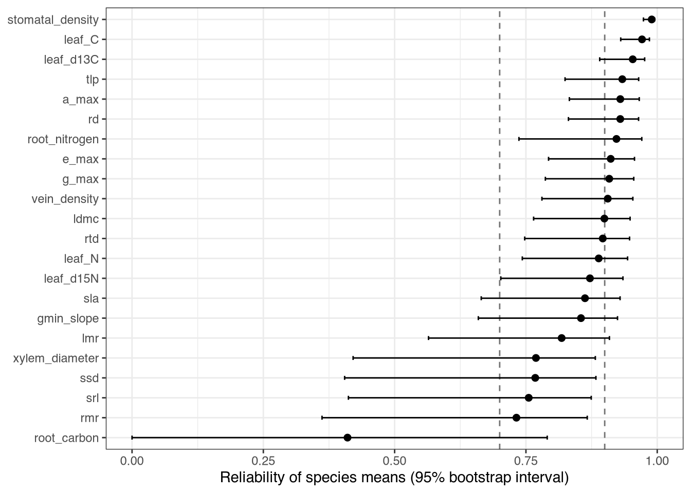
Below 0.9: lmr, rmr, gmin_slope, leaf_N, leaf_d15N, srl, rtd, root_carbon, sla, ldmc, ssd, xylem_diameter. Below 0.7: root_carbon. Species-trait combinations with fewer than three individuals: stomatal_density (CINMAL: n = 2), vein_density (OLEDIO: n = 1).
2.4 Species trait estimates
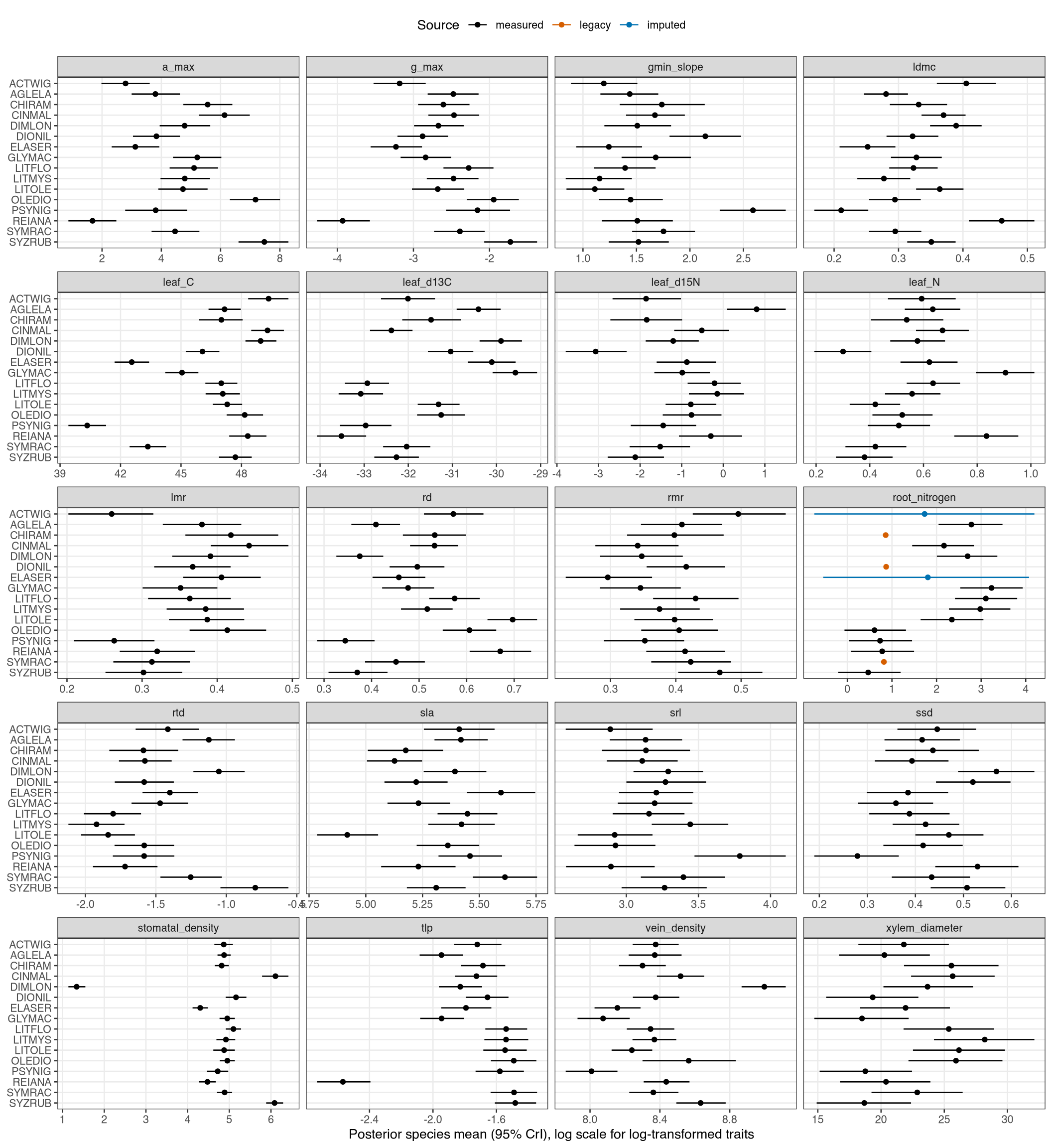
Species means are estimated, not averaged. For each trait, a hierarchical model of individual records (Gaussian, on the log scale for traits with skewness above 0.75 and strictly positive values: sla, srl, gmin_slope, leaf_N, g_max, rtd, stomatal_density, vein_density) gives a species intercept and, where plants have repeated records, an individual-within-species intercept. Each fit is re-run with more conservative sampler settings until R-hat < 1.01, bulk and tail ESS ≥ 400 and there are no divergent transitions. The posterior of each species intercept is the species estimate; 30 posterior draws of the full species × trait table are carried into the PCA so trait uncertainty can be checked downstream.
The figure shows posterior species means with 95% credible intervals on the modelling scale (log for the traits above). Species with few individuals have wide intervals and are pulled towards the across-species mean (partial pooling).
| Trait | Species with largest change | Simple mean | Posterior mean | Correlation across species |
|---|---|---|---|---|
| a_max | REIANA | 1.46 | 1.68 | 1.00 |
| g_max | SYZRUB | -1.42 | -1.73 | 0.99 |
| gmin_slope | CINMAL | 1.96 | 1.67 | 0.99 |
| ldmc | REIANA | 0.48 | 0.46 | 1.00 |
| leaf_C | PSYNIG | 40.12 | 40.35 | 1.00 |
| leaf_N | GLYMAC | 0.96 | 0.91 | 1.00 |
| leaf_d13C | REIANA | -33.63 | -33.52 | 1.00 |
| leaf_d15N | DIONIL | -3.34 | -3.07 | 1.00 |
| lmr | ACTWIG | 0.23 | 0.26 | 1.00 |
| rd | REIANA | 0.69 | 0.67 | 1.00 |
| rmr | ACTWIG | 0.54 | 0.50 | 1.00 |
| root_nitrogen | SYZRUB | 0.31 | 0.47 | 1.00 |
| rtd | SYZRUB | -0.66 | -0.79 | 1.00 |
| sla | ELASER | 5.89 | 5.60 | 0.97 |
| srl | PSYNIG | 4.06 | 3.79 | 0.98 |
| ssd | PSYNIG | 0.23 | 0.28 | 1.00 |
| stomatal_density | SYMRAC | 4.94 | 4.89 | 1.00 |
| tlp | REIANA | -2.66 | -2.57 | 1.00 |
| vein_density | OLEDIO | 8.64 | 8.57 | 1.00 |
| xylem_diameter | LITMYS | 30.05 | 28.20 | 1.00 |
Traits whose posterior means correlate below 0.95 with simple means: none.
All 21 trait models passed the convergence checks (max R-hat 1.008, min bulk ESS 450); models needing more conservative settings: sla (adapt_delta=0.99; max_treedepth=12; doubled warmup; sampling=2000; sampling=4000; sampling=8000; sampling=16000), ldmc (adapt_delta=0.99; max_treedepth=12; doubled warmup; sampling=2000; sampling=4000; sampling=8000; sampling=16000), stomatal_density (adapt_delta=0.99; max_treedepth=12; doubled warmup; sampling=2000).
Root nitrogen. Sources: imputed 2, legacy 3, measured 11 species. Imputed species take their value from a regression of root N on posterior-mean leaf N and SRL fitted across the species with root N; each draw table uses one posterior draw of the imputed value, so imputation uncertainty is carried forward.
| Term | Estimate [95% CrI] |
|---|---|
| Intercept | 0.61 [-6.73, 8.22] |
| leaf_N | 1.69 [-1.12, 4.32] |
| srl | 0.04 [-2.17, 2.18] |
| Species | Imputed root N [95% CrI] |
|---|---|
| ACTWIG | 1.73 [-0.74, 4.19] |
| ELASER | 1.81 [-0.54, 4.07] |
rootCN samples: 83 records, 83 mapped to species, 0 unmapped and excluded.
2.5 Covariation among traits
Species posterior means on the modelling scale (n = 16 species; a correlation needs to exceed about ±0.50 to be distinguishable from zero). Upper panels show Pearson r (shading increases with |r|) and pairwise n; lower panels show the species values; diagonals show distributions. LMR and RMR are compositional, so part of their correlation is built in.

3 Environment
| Measurement | Plots | Total plots | Percent | |
|---|---|---|---|---|
| canopy_cover | canopy_cover | 250 | 250 | 100.0 |
| soil_moisture | soil_moisture | 250 | 250 | 100.0 |
| soil_nutrients | soil_nutrients | 250 | 250 | 100.0 |
| temp_humidity | temp_humidity | 86 | 250 | 34.4 |
- Canopy:
canopy_coveriscanopy_open_2024, canopy openness in percent; higher values mean more light. It is labelled canopy openness in the PCA. - Temperature and humidity: only 86 plots have loggers, so they are left out of the environmental PCA and appear only in Models 5 and 6, which use that subset. 84,618 of 287,411 relative-humidity readings exceed 100%; these are retained in the cleaned data and included in the plot humidity means.
- Soil: organic carbon and nitrogen are almost collinear (r = 0.97), so nitrogen is dropped from the PCA and the models.

Same layout as the trait panel; temperature and humidity comparisons use only plots with loggers.


4 Principal component analyses
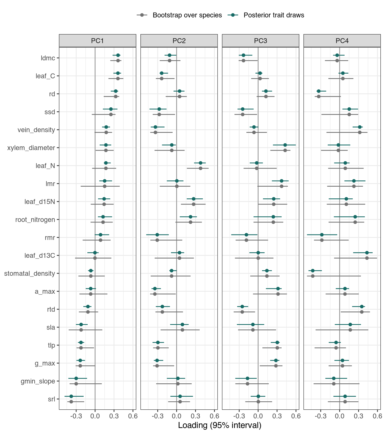
The main PCAs are the solutions the syndrome models use (secondary PCAs follow). Variables are standardised; the number of PCs is chosen by parallel analysis (Horn’s method, 95th percentile of eigenvalues from random data), and at least two are kept so every species and plot has PC1 and PC2 scores. Loading intervals come from bootstrapping species (or plots), with each resample rotated onto the reference solution. PC signs are arbitrary.
4.1 Traits
The trait PCA uses the posterior species means of 20 traits (a_max, g_max, gmin_slope, ldmc, leaf_C, leaf_d13C, leaf_d15N, leaf_N, lmr, rd, rmr, root_nitrogen, rtd, sla, srl, ssd, stomatal_density, tlp, vein_density, xylem_diameter).
Parallel analysis retains 4 PCs, explaining 72% of the variance. Strongest loadings: PC1: srl (-0.38), ldmc (+0.36), leaf_C (+0.36); PC2: leaf_N (+0.38), a_max (-0.34), vein_density (-0.34); PC3: xylem_diameter (+0.43), lmr (+0.37), a_max (+0.32); PC4: leaf_d13C (+0.43), stomatal_density (-0.43), rtd (+0.35).


4.1.1 Trait uncertainty in the PCA
The PCA is refitted to each of the 30 posterior trait tables and rotated onto the reference solution. If species scores barely move between draws, the scores used in the models are robust to uncertainty in the trait estimates; wide draw intervals mark species or loadings that depend on poorly estimated traits. Bootstrap intervals (resampling species) instead show how much the axes depend on which species were sampled.
| PC | Median r | Minimum r | Draws below threshold |
|---|---|---|---|
| PC1 | 0.983 | 0.945 | 0 |
| PC2 | 0.967 | 0.900 | 0 |
| PC3 | 0.948 | 0.703 | 1 |
| PC4 | 0.948 | 0.743 | 2 |
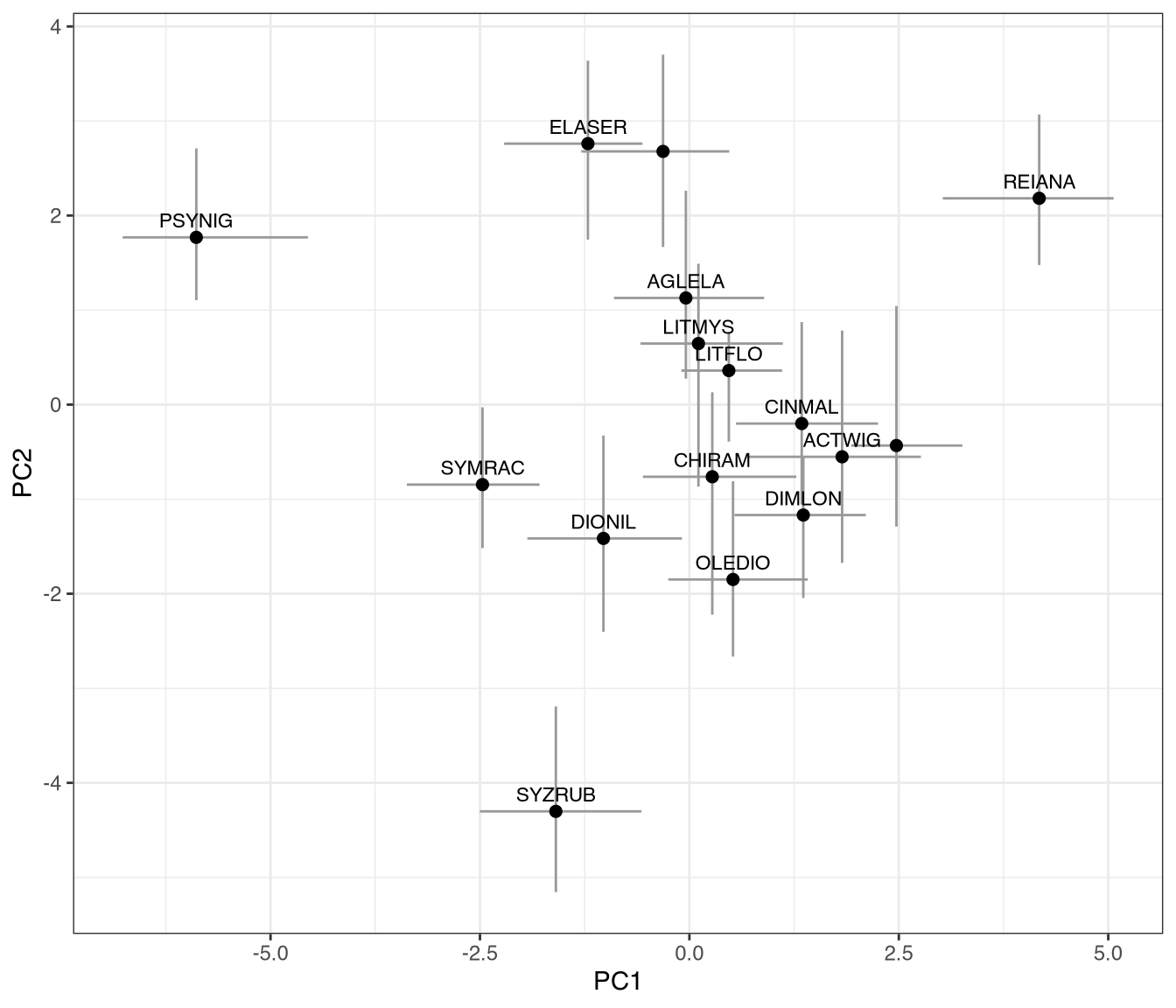
Species scores on the first two trait PCs (points) with the 95% range across posterior trait draws (grey bars).
4.2 Environment
The environmental PCA uses all plot variables except temperature, humidity and soil nitrogen, on the plots where every variable was measured; plots dropped for missing data: NCF_LX_P48.
Parallel analysis retains 2 PCs, explaining 53% of the variance. Strongest loadings: PC1: ph (-0.50), phosphorus (-0.49), potassium (-0.46); PC2: soil_moisture_var (-0.69), soil_moisture_mean (-0.61), phosphorus (+0.24).


4.3 Secondary PCAs
These PCAs are not used by the models. The trait-group PCAs show which traits within a functional group carry overlapping information, which helps decide which traits to keep as separate predictors: traits loading together on one axis are largely redundant, while a trait on its own axis adds independent information. The environmental PCAs show how plots spread along environmental gradients, including temperature and humidity (only plots with loggers) and soil nutrients alone. All use the same methods as the main PCAs.
4.3.1 Water-related traits
Parallel analysis retains 1 PC, explaining 46% of the variance. Strongest loadings: PC1: g_max (+0.56), a_max (+0.54), tlp (+0.53); PC2: gmin_slope (-0.70), xylem_diameter (+0.65), stomatal_density (-0.25).


4.3.2 Leaf traits
Parallel analysis retains 1 PC, explaining 36% of the variance. Strongest loadings: PC1: leaf_C (-0.59), ldmc (-0.56), vein_density (-0.43); PC2: leaf_N (+0.70), δ15N (+0.68), vein_density (-0.22).


4.3.3 Root traits
Parallel analysis retains 1 PC, explaining 53% of the variance. Strongest loadings: PC1: rd (+0.67), srl (-0.52), rtd (-0.50); PC2: root_nitrogen (-0.85), srl (-0.37), rtd (+0.34).


4.3.4 Environment including temperature and humidity (plots with loggers)
Parallel analysis retains 3 PCs, explaining 56% of the variance. Strongest loadings: PC1: phosphorus (-0.44), ph (-0.41), potassium (-0.39); PC2: soil_moisture_var (-0.57), soil_moisture_mean (-0.49), humidity_var (-0.46); PC3: canopy_openness (-0.45), temperature_var (-0.40), temperature_mean (-0.36).


4.3.5 Soil nutrients
Parallel analysis retains 1 PC, explaining 50% of the variance. Strongest loadings: PC1: phosphorus (-0.55), ph (-0.52), potassium (-0.51); PC2: organiccarbon (+0.74), ph (-0.50), phosphorus (-0.34).


5 Models
All models share the same structure. The census interval enters as an
offset, offset(log(interval)), so population-level
coefficients are log hazard ratios (mortality: binomial with
complementary log-log link) or log rate ratios (recruitment: negative
binomial with log link) per standard deviation of each predictor. Every
model has species random intercepts and species-specific slopes on the
environmental predictors, and random intercepts for plot within site and
for census date. Models are fitted in Stan through brms
with 4 chains of 1000 iterations (250 warmup), set in
config.yml.
A ratio above 1 means a higher death (or recruitment) rate per SD increase in the predictor. Posterior predictive checks compare observed death or recruit totals with totals simulated from the model, overall and for each site and census date.
| Model | Status | Family | Rows | Divergences | Max R-hat | Min ESS (bulk/tail) | PPC total within 95% | PPC sites / dates within 95% |
|---|---|---|---|---|---|---|---|---|
| 1: mortality, syndromes | fitted | binomial (cloglog) | 6,390 | 1 | 1.003 | 2362/2857 | yes | 6/6 / 7/7 |
| 2: recruitment, syndromes | fitted | negbinomial (log) | 26,912 | 0 | 1.002 | 2110/3223 | yes | 6/6 / 7/7 |
| 3: mortality, mechanistic | fitted | binomial (cloglog) | 6,390 | 0 | 1.002 | 2251/2373 | yes | 6/6 / 7/7 |
| 4: recruitment, mechanistic | fitted | negbinomial (log) | 26,912 | 0 | 1.003 | 2061/1944 | yes | 6/6 / 7/7 |
| 5: mortality, mechanistic + climate | fitted | binomial (cloglog) | 2,222 | 0 | 1.002 | 1949/2422 | yes | 6/6 / 7/7 |
| 6: recruitment, mechanistic + climate | fitted | negbinomial (log) | 9,232 | 0 | 1.002 | 1717/1706 | yes | 6/6 / 7/7 |
5.1 Syndrome models
The syndrome models ask whether species’ overall trait strategies (trait PCs) and plots’ overall environments (environmental PCs) predict demography. They use the 4 retained trait PCs (72% of trait variance) and 2 environmental PCs (53% of environmental variance), with no trait × environment interactions. PC scores are rescaled to unit SD. Priors: normal(0, 1) on the intercept and fixed effects, exponential(1) on group-level SDs (and on the negative-binomial shape). Species slopes on the environmental PCs are uncorrelated.
5.1.1 Model 1: mortality
Deaths among individuals at risk in each plot × species × census interval × cohort, with age and plot density as covariates alongside the trait and environmental PCs.
Fit: binomial (cloglog), 6,390 rows; 4 chains x 4000 iterations (2000 warmup); 1 divergent transitions; max R-hat 1.003; min bulk/tail ESS 2362/2857.
Formula:
deaths | trials(n) ~ age + density + trait_PC1 + trait_PC2 + trait_PC3 + trait_PC4 + env_PC1 + env_PC2 + offset(log(interval)) + (1 + env_PC1 + env_PC2 || species) + (1 | plot_id:division) + (1 | date)
| Group | Term | Hazard ratio [95% CrI] | Excludes 1 |
|---|---|---|---|
| Demography | Age | 0.53 [0.50, 0.55] | yes |
| Demography | Density | 1.00 [0.97, 1.03] | |
| Trait PCs | Trait PC1 | 0.78 [0.61, 0.99] | yes |
| Trait PCs | Trait PC2 | 0.81 [0.63, 1.05] | |
| Trait PCs | Trait PC3 | 1.01 [0.78, 1.31] | |
| Trait PCs | Trait PC4 | 0.93 [0.72, 1.20] | |
| Environmental PCs | Env PC1 | 1.04 [0.95, 1.13] | |
| Environmental PCs | Env PC2 | 0.98 [0.87, 1.08] |

Posterior predictive check: observed total 5,616 vs predicted 5,633 [5,481, 5,774]; site totals inside the 95% interval: 6/6; census-date totals: 7/7.


| Predictor | Change per +1 SD at the median [95% CrI] |
|---|---|
| age | -0.1933 [-0.2292, -0.1562] |
| density | 0.0002 [-0.0075, 0.0078] |
| trait_PC1 | -0.0705 [-0.1474, -0.0013] |
| trait_PC2 | -0.0584 [-0.1267, 0.0150] |
| trait_PC3 | 0.0040 [-0.0749, 0.0731] |
| trait_PC4 | -0.0218 [-0.0995, 0.0485] |
| env_PC1 | 0.0117 [-0.0131, 0.0362] |
| env_PC2 | -0.0067 [-0.0380, 0.0218] |
| Group | Parameter | Estimate [95% CrI] | R-hat |
|---|---|---|---|
| date | sd(Intercept) | 0.38 [0.20, 0.70] | 1.001 |
| plot_id:division | sd(Intercept) | 0.51 [0.45, 0.58] | 1.001 |
| species | sd(Intercept) | 0.47 [0.28, 0.78] | 1.000 |
| species | sd(env_PC1) | 0.04 [0.00, 0.13] | 1.003 |
| species | sd(env_PC2) | 0.09 [0.01, 0.20] | 1.001 |
5.1.2 Model 2: recruitment
Recruits per plot × species × census interval, including zeros for focal species not recruiting in a plot. Density is the plot density at the previous census. Each site’s first census is dropped.
Fit: negbinomial (log), 26,912 rows; 4 chains x 4000 iterations (2000 warmup); 0 divergent transitions; max R-hat 1.002; min bulk/tail ESS 2110/3223.
Formula:
recruit_count ~ density + trait_PC1 + trait_PC2 + trait_PC3 + trait_PC4 + env_PC1 + env_PC2 + offset(log(interval)) + (1 + env_PC1 + env_PC2 || species) + (1 | plot_id:division) + (1 | date)
| Group | Term | Rate ratio [95% CrI] | Excludes 1 |
|---|---|---|---|
| Demography | Density | 1.12 [1.01, 1.23] | yes |
| Trait PCs | Trait PC1 | 0.75 [0.39, 1.46] | |
| Trait PCs | Trait PC2 | 0.96 [0.51, 1.81] | |
| Trait PCs | Trait PC3 | 0.67 [0.35, 1.33] | |
| Trait PCs | Trait PC4 | 1.13 [0.58, 2.15] | |
| Environmental PCs | Env PC1 | 0.91 [0.75, 1.14] | |
| Environmental PCs | Env PC2 | 1.00 [0.83, 1.20] |

Posterior predictive check: observed total 4,622 vs predicted 4,714 [3,795, 6,377]; site totals inside the 95% interval: 6/6; census-date totals: 7/7.


| Predictor | Change per +1 SD at the median [95% CrI] |
|---|---|
| trait_PC1 | -0.0930 [-0.4815, 0.1546] |
| trait_PC2 | -0.0104 [-0.3656, 0.2583] |
| trait_PC3 | -0.1297 [-0.6053, 0.1056] |
| trait_PC4 | 0.0392 [-0.2612, 0.3463] |
| env_PC1 | -0.0300 [-0.1542, 0.0521] |
| env_PC2 | -0.0000 [-0.0907, 0.0931] |
| Group | Parameter | Estimate [95% CrI] | R-hat |
|---|---|---|---|
| date | sd(Intercept) | 1.73 [0.88, 3.05] | 1.001 |
| plot_id:division | sd(Intercept) | 0.97 [0.83, 1.13] | 1.000 |
| species | sd(Intercept) | 1.68 [1.11, 2.60] | 1.002 |
| species | sd(env_PC1) | 0.27 [0.12, 0.47] | 1.001 |
| species | sd(env_PC2) | 0.20 [0.08, 0.35] | 1.001 |
| Family | shape | 0.09 [0.08, 0.10] | 1.001 |
5.2 Mechanistic models
The mechanistic models replace the PCs with individual traits and environmental variables and test three trait × environment interactions, each a hypothesised mechanism:
- canopy openness × SLA: light capture; high-SLA species may gain more from open canopy.
- soil moisture × TLP: drought tolerance; species with lower (more negative) turgor loss points may suffer less in dry plots.
- phosphorus × SRL: nutrient foraging; high-SRL species may respond more to soil phosphorus.
Main effects are SLA, TLP, RMR, SRL and SSD (traits) and canopy openness, mean soil moisture and phosphorus (environment), plus age and density for mortality and density for recruitment. Species have random slopes on the three environmental variables. Priors are tighter than in the syndrome models: normal(0, 0.5) on the intercept and fixed effects and exponential(2) on group-level SDs (exponential(1) on the negative-binomial shape).
For mortality, with \(Y_i\) deaths among \(n_i\) at risk over \(\Delta t_i\) years:
\[ \begin{aligned} Y_i \mid n_i &\sim \operatorname{Binomial}(n_i,\, p_i), \\ \operatorname{cloglog}(p_i) &= \log \Delta t_i + \beta_0 + \beta_a a_i + \beta_\rho \rho_i + \boldsymbol{\beta}_E^{\top}\mathbf{E}_{p[i]} + \boldsymbol{\beta}_T^{\top}\mathbf{T}_{s[i]} \\ &\quad + \delta_1 C_{p[i]}\,\mathrm{SLA}_{s[i]} + \delta_2 M_{p[i]}\,\mathrm{TLP}_{s[i]} + \delta_3 P_{p[i]}\,\mathrm{SRL}_{s[i]} \\ &\quad + b_{0,s[i]} + b_{C,s[i]} C_{p[i]} + b_{M,s[i]} M_{p[i]} + b_{P,s[i]} P_{p[i]} + u_{p[i]:d[i]} + v_{t[i]}, \end{aligned} \]
where \(a\) is age, \(\rho\) density, \(\mathbf{E} = (C, M, P)\) canopy openness, soil moisture and phosphorus, \(\mathbf{T}\) the five traits, and \(s\), \(p\), \(d\), \(t\) index species, plot, site and census date. The cumulative hazard over the interval is \(\Delta t_i h_i\) and \(p_i = 1 - \exp(-\Delta t_i h_i)\), so \(\exp(\beta)\) is a hazard ratio. Recruitment uses the same linear predictor without age, with \(R_i \sim \operatorname{NegBinomial}(\lambda_i, \phi)\) and \(\log \lambda_i\) in place of \(\operatorname{cloglog}(p_i)\).
Models 3 and 4 treat the species intercept and slopes as independent normal effects. Models 5 and 6 add mean temperature and humidity as fixed effects, which restricts them to plots with loggers; Model 5 also lets the species intercept and slopes correlate, \((b_{0,s}, b_{C,s}, b_{M,s}, b_{P,s})^{\top} \sim \operatorname{MVN}(\mathbf{0}, \boldsymbol{\Sigma})\) with an LKJ(2) prior on the correlations.
5.2.1 Reading the interaction results
The interaction coefficient \(\delta\) is the formal test, on the link scale: the log-hazard scale (cloglog) for mortality and the log-rate scale for recruitment. A species’ environmental slope on that scale is \(\beta_E + \delta \cdot \text{trait}_s + b_{E,s}\): the population slope, shifted by the species’ trait through \(\delta\), plus the species’ own deviation \(b_{E,s}\). Each model is shown with four figures.
- Species effects against trait value (main figure). For each species, the predicted change in 1-year mortality probability (or recruits per year) when the environmental variable rises from its mean by 1 SD, holding everything else constant: other environmental variables, age and density at their means, the species at its own trait values and with its own species effects. The line and band are the same quantity for a hypothetical species across the trait range, with other traits at their mean and no species effects. The tilt of the line reflects the interaction; how closely the species follow it shows how much of their variation the trait explains; outlying points show which species drive the result. Because these are response-scale effects, species also differ through their baseline mortality (intercepts and other traits), not only through the trait on the x-axis. The table gives the SD of the species’ own environmental slopes on the link scale: when it is small, species differ little in their environmental response beyond what the fixed effects imply.
- Environmental effect as a function of trait. The population ratio per SD of environment across the observed trait range, with its 95% band. Shading marks the trait range where the band excludes 1 (a Johnson–Neyman region: the kinds of species for which the environment has a detectable effect), the dotted line the trait value where the posterior-mean ratio equals 1 (shown only when the band excludes 1 somewhere), and ticks the species’ trait values, i.e. where the curve is supported by data.
- Reaction norms on the response scale. Predicted 1-year mortality probability (or recruits per year) across the observed environmental range, for the 10th, 50th and 90th percentiles of the trait among species (population level, other predictors at their mean) and for the two real species at the trait extremes (including their own species effects). This is what plants experience, but it is a different scale from \(\delta\): on the probability scale curves converge or diverge even when \(\delta = 0\), because baseline mortality differs between species. Statements about the interaction refer to the link scale; statements about mortality or recruitment levels refer to this figure.
- Trait × environment surface (supplementary). The population-level prediction over the trait and environment space with the observed species × plot combinations overlaid; areas outside their convex hull are greyed out because, with 16 species, much of the space is extrapolation.
The model scripts also save marginal-effect slope figures and
per-species changes per SD at each species’ observed conditions
(*_slopes.png, *_species_env_1sd_changes.png);
the species-effect figure above supersedes them in the report.
5.2.2 Causal assumptions
The DAGs encode the assumed causal structure; the adjustment sets
below are computed from them with dagitty and hold only
under those assumptions. Two points matter for interpretation. Traits
vary only between species, so a species-level adjustment leaves little
variation to identify trait effects; the models use partially pooled
species intercepts rather than fixed species effects, so trait effects
are estimated from the 16 species with correspondingly wide intervals.
Density lies downstream of the environment, so conditioning on density
estimates environmental effects not mediated by density rather than
total effects.

| Exposure | Minimal adjustment sets |
|---|---|
| allocation_traits | species |
| canopy_cover | date, plot |
| canopy_cover_leaf_traits_interaction | canopy_cover, leaf_traits |
| humidity | date, plot |
| leaf_traits | species |
| other_traits | species |
| root_traits | species |
| soil_moisture | date, plot |
| soil_moisture_root_traits_interaction | root_traits, soil_moisture |
| soil_moisture_water_traits_interaction | soil_moisture, water_traits |
| soil_nutrients | date, plot |
| soil_nutrients_root_traits_interaction | root_traits, soil_nutrients |
| temperature | date, plot |
| water_traits | species |
5.2.3 Model 3: mortality
Fit: binomial (cloglog), 6,390 rows; 4 chains x 4000 iterations (2000 warmup); 0 divergent transitions; max R-hat 1.002; min bulk/tail ESS 2251/2373.
Formula:
deaths | trials(n) ~ offset(log(interval)) + age + density + canopy_cover + soil_moisture_mean + phosphorus + sla + tlp + rmr + srl + ssd + canopy_cover:sla + soil_moisture_mean:tlp + phosphorus:srl + (1 + canopy_cover + soil_moisture_mean + phosphorus || species) + (1 | plot_id:division) + (1 | date)
| Group | Term | Hazard ratio [95% CrI] | Excludes 1 |
|---|---|---|---|
| Demography | age | 0.53 [0.51, 0.55] | yes |
| Demography | density | 1.00 [0.97, 1.03] | |
| Environment | canopy_cover | 0.90 [0.79, 1.01] | |
| Environment | soil_moisture_mean | 0.95 [0.87, 1.05] | |
| Environment | phosphorus | 0.96 [0.88, 1.05] | |
| Traits | sla | 1.11 [0.83, 1.48] | |
| Traits | tlp | 1.13 [0.85, 1.51] | |
| Traits | rmr | 1.26 [0.94, 1.68] | |
| Traits | srl | 1.17 [0.84, 1.62] | |
| Traits | ssd | 0.92 [0.69, 1.22] | |
| Interactions | canopy_cover x sla | 0.92 [0.82, 1.03] | |
| Interactions | soil_moisture_mean x tlp | 0.96 [0.91, 1.01] | |
| Interactions | phosphorus x srl | 1.01 [0.98, 1.06] |

Posterior predictive check: observed total 5,616 vs predicted 5,625 [5,478, 5,775]; site totals inside the 95% interval: 6/6; census-date totals: 7/7.


| Predictor | Change per +1 SD at the median [95% CrI] |
|---|---|
| age | -0.1906 [-0.2268, -0.1539] |
| density | -0.0004 [-0.0082, 0.0072] |
| canopy_cover | -0.0279 [-0.0677, 0.0020] |
| soil_moisture_mean | -0.0138 [-0.0384, 0.0131] |
| phosphorus | -0.0105 [-0.0363, 0.0140] |
| sla | 0.0289 [-0.0517, 0.1218] |
| tlp | 0.0363 [-0.0433, 0.1304] |
| rmr | 0.0567 [-0.0190, 0.1152] |
| srl | 0.0447 [-0.0484, 0.1496] |
| ssd | -0.0215 [-0.1091, 0.0546] |
| Group | Parameter | Estimate [95% CrI] | R-hat |
|---|---|---|---|
| date | sd(Intercept) | 0.37 [0.20, 0.70] | 1.001 |
| plot_id:division | sd(Intercept) | 0.50 [0.44, 0.58] | 1.000 |
| species | sd(Intercept) | 0.46 [0.28, 0.75] | 1.000 |
| species | sd(canopy_cover) | 0.10 [0.02, 0.23] | 1.002 |
| species | sd(soil_moisture_mean) | 0.05 [0.00, 0.15] | 1.002 |
| species | sd(phosphorus) | 0.03 [0.00, 0.10] | 1.001 |

| Environment | SD [95% CrI] |
|---|---|
| canopy_cover | 0.10 [0.02, 0.23] |
| soil_moisture_mean | 0.04 [0.00, 0.15] |
| phosphorus | 0.03 [0.00, 0.10] |
| Interaction | Trait range where the 95% band excludes 1 | Direction | Ratio = 1 at trait value |
|---|---|---|---|
| canopy_cover x sla | 0.08 to 1.57 | ratio < 1 | -1.19 |
| soil_moisture_mean x tlp | none | ||
| phosphorus x srl | none |


Supplementary: predicted response over the trait x environment space.

5.2.4 Model 4: recruitment
Fit: negbinomial (log), 26,912 rows; 4 chains x 4000 iterations (2000 warmup); 0 divergent transitions; max R-hat 1.003; min bulk/tail ESS 2061/1944.
Formula:
recruit_count ~ offset(log(interval)) + density + canopy_cover + soil_moisture_mean + phosphorus + sla + tlp + rmr + srl + ssd + canopy_cover:sla + soil_moisture_mean:tlp + phosphorus:srl + (1 + canopy_cover + soil_moisture_mean + phosphorus || species) + (1 | plot_id:division) + (1 | date)
| Group | Term | Rate ratio [95% CrI] | Excludes 1 |
|---|---|---|---|
| Demography | density | 1.12 [1.02, 1.24] | yes |
| Environment | canopy_cover | 1.08 [0.87, 1.34] | |
| Environment | soil_moisture_mean | 1.20 [0.99, 1.46] | |
| Environment | phosphorus | 1.12 [0.93, 1.34] | |
| Traits | sla | 1.10 [0.59, 2.16] | |
| Traits | tlp | 0.86 [0.45, 1.70] | |
| Traits | rmr | 1.21 [0.61, 2.32] | |
| Traits | srl | 1.73 [0.81, 3.50] | |
| Traits | ssd | 1.07 [0.54, 2.09] | |
| Interactions | canopy_cover x sla | 0.93 [0.77, 1.13] | |
| Interactions | soil_moisture_mean x tlp | 0.99 [0.84, 1.15] | |
| Interactions | phosphorus x srl | 1.08 [0.94, 1.23] |

Posterior predictive check: observed total 4,622 vs predicted 4,570 [3,771, 6,056]; site totals inside the 95% interval: 6/6; census-date totals: 7/7.


| Predictor | Change per +1 SD at the median [95% CrI] |
|---|---|
| density | 0.0401 [0.0060, 0.1344] |
| canopy_cover | 0.0253 [-0.0628, 0.1581] |
| soil_moisture_mean | 0.0651 [-0.0034, 0.2412] |
| phosphorus | 0.0399 [-0.0295, 0.1835] |
| sla | 0.0317 [-0.2442, 0.4954] |
| tlp | -0.0485 [-0.4002, 0.2682] |
| rmr | 0.0722 [-0.2246, 0.5308] |
| srl | 0.1869 [-0.0880, 0.7394] |
| ssd | 0.0226 [-0.3191, 0.3680] |
| Group | Parameter | Estimate [95% CrI] | R-hat |
|---|---|---|---|
| date | sd(Intercept) | 1.77 [0.88, 3.12] | 1.003 |
| plot_id:division | sd(Intercept) | 0.93 [0.78, 1.09] | 1.001 |
| species | sd(Intercept) | 1.65 [1.06, 2.55] | 1.001 |
| species | sd(canopy_cover) | 0.30 [0.16, 0.49] | 1.000 |
| species | sd(soil_moisture_mean) | 0.24 [0.10, 0.43] | 1.002 |
| species | sd(phosphorus) | 0.20 [0.05, 0.39] | 1.001 |
| Family | shape | 0.09 [0.08, 0.10] | 1.001 |

| Environment | SD [95% CrI] |
|---|---|
| canopy_cover | 0.29 [0.16, 0.49] |
| soil_moisture_mean | 0.23 [0.10, 0.43] |
| phosphorus | 0.19 [0.05, 0.39] |
| Interaction | Trait range where the 95% band excludes 1 | Direction | Ratio = 1 at trait value |
|---|---|---|---|
| canopy_cover x sla | none | ||
| soil_moisture_mean x tlp | none | ||
| phosphorus x srl | none |


Supplementary: predicted response over the trait x environment space.

5.2.5 Model 5: mortality with temperature and humidity
Fit: binomial (cloglog), 2,222 rows; 4 chains x 4000 iterations (2000 warmup); 0 divergent transitions; max R-hat 1.002; min bulk/tail ESS 1949/2422.
Formula:
deaths | trials(n) ~ offset(log(interval)) + age + density + canopy_cover + soil_moisture_mean + phosphorus + temperature_mean + humidity_mean + sla + tlp + rmr + srl + ssd + canopy_cover:sla + soil_moisture_mean:tlp + phosphorus:srl + (1 + canopy_cover + soil_moisture_mean + phosphorus | species) + (1 | plot_id:division) + (1 | date)
| Group | Term | Hazard ratio [95% CrI] | Excludes 1 |
|---|---|---|---|
| Demography | age | 0.55 [0.51, 0.59] | yes |
| Demography | density | 0.98 [0.95, 1.02] | |
| Environment | canopy_cover | 0.85 [0.72, 0.98] | yes |
| Environment | soil_moisture_mean | 0.85 [0.70, 1.02] | |
| Environment | phosphorus | 1.03 [0.86, 1.24] | |
| Environment | temperature_mean | 1.09 [0.92, 1.29] | |
| Environment | humidity_mean | 0.85 [0.74, 0.97] | yes |
| Traits | sla | 1.08 [0.74, 1.59] | |
| Traits | tlp | 1.26 [0.87, 1.77] | |
| Traits | rmr | 1.36 [0.95, 1.91] | |
| Traits | srl | 1.17 [0.79, 1.75] | |
| Traits | ssd | 1.02 [0.73, 1.40] | |
| Interactions | canopy_cover x sla | 0.96 [0.82, 1.10] | |
| Interactions | soil_moisture_mean x tlp | 0.90 [0.79, 1.01] | |
| Interactions | phosphorus x srl | 1.02 [0.93, 1.14] |

Posterior predictive check: observed total 2,383 vs predicted 2,388 [2,284, 2,486]; site totals inside the 95% interval: 6/6; census-date totals: 7/7.


| Predictor | Change per +1 SD at the median [95% CrI] |
|---|---|
| age | -0.1827 [-0.2244, -0.1415] |
| density | -0.0051 [-0.0159, 0.0045] |
| canopy_cover | -0.0458 [-0.0982, -0.0049] |
| soil_moisture_mean | -0.0491 [-0.1083, 0.0056] |
| phosphorus | 0.0072 [-0.0444, 0.0645] |
| temperature_mean | 0.0242 [-0.0246, 0.0724] |
| humidity_mean | -0.0450 [-0.0853, -0.0070] |
| sla | 0.0218 [-0.0812, 0.1479] |
| tlp | 0.0708 [-0.0368, 0.1915] |
| rmr | 0.0742 [-0.0149, 0.1439] |
| srl | 0.0470 [-0.0674, 0.1770] |
| ssd | 0.0061 [-0.0942, 0.0980] |
| Group | Parameter | Estimate [95% CrI] | R-hat |
|---|---|---|---|
| date | sd(Intercept) | 0.37 [0.20, 0.71] | 1.001 |
| plot_id:division | sd(Intercept) | 0.54 [0.42, 0.68] | 1.000 |
| species | sd(Intercept) | 0.58 [0.30, 1.01] | 1.002 |
| species | sd(canopy_cover) | 0.08 [0.00, 0.25] | 1.001 |
| species | sd(soil_moisture_mean) | 0.15 [0.01, 0.39] | 1.001 |
| species | sd(phosphorus) | 0.12 [0.01, 0.32] | 1.001 |
| species | cor(Intercept,canopy_cover) | 0.01 [-0.68, 0.69] | 1.000 |
| species | cor(Intercept,soil_moisture_mean) | 0.10 [-0.56, 0.71] | 1.001 |
| species | cor(canopy_cover,soil_moisture_mean) | -0.02 [-0.71, 0.69] | 1.000 |
| species | cor(Intercept,phosphorus) | 0.13 [-0.56, 0.75] | 1.001 |
| species | cor(canopy_cover,phosphorus) | -0.05 [-0.74, 0.68] | 1.000 |
| species | cor(soil_moisture_mean,phosphorus) | 0.19 [-0.57, 0.81] | 1.000 |

| Environment | SD [95% CrI] |
|---|---|
| canopy_cover | 0.06 [0.00, 0.25] |
| soil_moisture_mean | 0.13 [0.01, 0.39] |
| phosphorus | 0.11 [0.01, 0.32] |
| Interaction | Trait range where the 95% band excludes 1 | Direction | Ratio = 1 at trait value |
|---|---|---|---|
| canopy_cover x sla | -0.20 to 1.41 | ratio < 1 | |
| soil_moisture_mean x tlp | 0.20 to 0.88 | ratio < 1 | -1.62 |
| phosphorus x srl | none |


Supplementary: predicted response over the trait x environment space.

5.2.6 Model 6: recruitment with temperature and humidity
Fit: negbinomial (log), 9,232 rows; 4 chains x 4000 iterations (2000 warmup); 0 divergent transitions; max R-hat 1.002; min bulk/tail ESS 1717/1706.
Formula:
recruit_count ~ offset(log(interval)) + density + canopy_cover + soil_moisture_mean + phosphorus + temperature_mean + humidity_mean + sla + tlp + rmr + srl + ssd + canopy_cover:sla + soil_moisture_mean:tlp + phosphorus:srl + (1 + canopy_cover + soil_moisture_mean + phosphorus || species) + (1 | plot_id:division) + (1 | date)
| Group | Term | Rate ratio [95% CrI] | Excludes 1 |
|---|---|---|---|
| Demography | density | 1.14 [0.97, 1.34] | |
| Environment | canopy_cover | 1.09 [0.85, 1.38] | |
| Environment | soil_moisture_mean | 1.32 [0.90, 1.92] | |
| Environment | phosphorus | 1.08 [0.79, 1.46] | |
| Environment | temperature_mean | 0.73 [0.55, 0.97] | yes |
| Environment | humidity_mean | 1.00 [0.79, 1.29] | |
| Traits | sla | 1.12 [0.55, 2.28] | |
| Traits | tlp | 0.94 [0.47, 1.88] | |
| Traits | rmr | 1.14 [0.54, 2.26] | |
| Traits | srl | 1.72 [0.77, 3.70] | |
| Traits | ssd | 1.08 [0.53, 2.21] | |
| Interactions | canopy_cover x sla | 0.90 [0.74, 1.10] | |
| Interactions | soil_moisture_mean x tlp | 0.92 [0.66, 1.28] | |
| Interactions | phosphorus x srl | 1.10 [0.90, 1.37] |

Posterior predictive check: observed total 2,219 vs predicted 2,352 [1,505, 4,325]; site totals inside the 95% interval: 6/6; census-date totals: 7/7.


| Predictor | Change per +1 SD at the median [95% CrI] |
|---|---|
| density | 0.0431 [-0.0107, 0.1690] |
| canopy_cover | 0.0297 [-0.0760, 0.1760] |
| soil_moisture_mean | 0.0895 [-0.0387, 0.3509] |
| phosphorus | 0.0259 [-0.1112, 0.2016] |
| temperature_mean | -0.1181 [-0.4193, -0.0078] |
| humidity_mean | 0.0013 [-0.1137, 0.1344] |
| sla | 0.0369 [-0.2600, 0.5124] |
| tlp | -0.0206 [-0.3423, 0.3297] |
| rmr | 0.0459 [-0.2664, 0.4881] |
| srl | 0.1831 [-0.1059, 0.7702] |
| ssd | 0.0250 [-0.3329, 0.3824] |
| Group | Parameter | Estimate [95% CrI] | R-hat |
|---|---|---|---|
| date | sd(Intercept) | 1.66 [0.79, 3.06] | 1.002 |
| plot_id:division | sd(Intercept) | 0.91 [0.62, 1.22] | 1.001 |
| species | sd(Intercept) | 1.85 [1.16, 2.96] | 1.001 |
| species | sd(canopy_cover) | 0.17 [0.01, 0.43] | 1.001 |
| species | sd(soil_moisture_mean) | 0.57 [0.28, 0.97] | 1.000 |
| species | sd(phosphorus) | 0.27 [0.02, 0.60] | 1.002 |
| Family | shape | 0.08 [0.06, 0.09] | 1.000 |

| Environment | SD [95% CrI] |
|---|---|
| canopy_cover | 0.16 [0.01, 0.43] |
| soil_moisture_mean | 0.56 [0.28, 0.97] |
| phosphorus | 0.26 [0.02, 0.60] |
| Interaction | Trait range where the 95% band excludes 1 | Direction | Ratio = 1 at trait value |
|---|---|---|---|
| canopy_cover x sla | none | ||
| soil_moisture_mean x tlp | none | ||
| phosphorus x srl | none |


Supplementary: predicted response over the trait x environment space.
